18 Artificial Intelligence
This chapter is supplementary reading. It covers AI and neural networks in more depth than the core course requires. Read it if the topic interests you, or return to it when these ideas come up elsewhere in your studies. Some of it is quite advanced, and since it is still in progress, read for interest only.
18.1 What is Artificial Intelligence?
Artificial intelligence (AI) is the project of building systems that perform tasks which, in humans, require intelligence: perception, learning, language use, reasoning, planning, and decision making. The term was introduced in the 1955 Dartmouth proposal, which framed the goal as describing aspects of intelligence precisely enough that a machine could simulate them (McCarthy et al., 1955).
AI can be treated as engineering or as theory of mind. An engineering system may work without matching human cognition; a cognitive model aims to explain behaviour and mechanism. Psychology draws on both: AI methods can be tools, and they can serve as models of representation and processing.
In 1950, Alan Turing proposed a practical approach to the question. Rather than asking “Can machines think?”, a question that gets stuck on definitions, he proposed the imitation game: a human interrogator communicates by text with two hidden partners, one human and one machine. If the machine can fool the interrogator consistently, Turing argued, we have as much reason to call it intelligent as we do a person. The test sidesteps philosophical debates and focuses on observable performance. The imitation game (now commonly called the Turing test) set the tone for a field that judges intelligence by what a system can do. (Turing, 1950)
18.2 A brief history of the idea
Long before electronic computers, Charles Babbage designed calculating machines in the 1820s and 1830s. His Analytical Engine anticipated the architecture of modern computers: it had a memory store, a processing unit, and punched cards for programming, borrowed from the Jacquard loom. Ada Lovelace, working with Babbage, argued in 1843 that such a machine could manipulate any symbols that could be formally represented, not just numbers. These ideas anticipated the architecture of modern computers even though the machines were never completed. (Science Museum Group, n.d.)
By mid-20th century, Turing’s 1950 paper had reframed the problem as a test of behaviour. The next landmark was the Dartmouth workshop proposal of 1955. John McCarthy, Marvin Minsky, Nathaniel Rochester, and Claude Shannon wrote a funding proposal stating that “every aspect of learning or any other feature of intelligence can in principle be so precisely described that a machine can be made to simulate it.” The workshop, held in 1956, gave the field its name and established its core agenda: making machines that could use language, form abstractions, solve problems, and improve themselves. Many of the attendees led AI research for decades. (McCarthy et al., 1955)
Early AI work emphasised symbolic problem solving and rule-based reasoning. Intelligence was framed as the manipulation of symbols according to explicit rules. The key technical challenges were representation (encoding knowledge in a form the machine can work with) and search (navigating large spaces of possible actions). This approach produced demonstrations in games, theorem proving, and planning. But the real world is noisy, ambiguous, and incomplete. Machine translation was an early casualty: researchers discovered that translating natural language required not just grammar rules but vast world knowledge, and progress stalled. Expert systems in the 1970s and 1980s attempted to capture specialist knowledge as explicit rules. MYCIN, for example, encoded hundreds of rules for diagnosing bacterial infections. These systems worked in narrow domains but were brittle: they failed when they encountered situations their rules did not cover, even slightly novel ones. The resulting disappointment contributed to the AI winters: periods of sharply reduced funding and public confidence. A first AI winter struck in the mid-1970s; a second in the late 1980s. (McCorduck, 2004; Nilsson, 2010)
Running in parallel was a different approach rooted in associationism: the philosophical tradition holding that complex mental life arises from the association of simple elements. In modern form, those elements are artificial neurons connected by adjustable links. This connectionist approach is bottom-up: rather than programming rules, you specify a network architecture and a learning procedure, and the system finds its own rules from examples. The distinction matters. is top-down: the programmer specifies the rules and the machine follows them. The connectionist approach is bottom-up: the programmer specifies a network and a learning procedure, and the system discovers its own representations by being exposed to examples. The knowledge lives not in explicit rules but in the pattern of connection strengths across many units. (Nilsson, 2010)
Early milestones: McCulloch and Pitts (1943) modelled neurons as logical devices; Hebb (1949) proposed that experience strengthens synaptic connections; Rosenblatt (1958) built the , the first practical learning machine. Minsky and Papert’s 1969 analysis showed that single-layer perceptrons had fundamental limits, cooling interest for a decade. The revival came in 1986 when Rumelhart, Hinton, and Williams demonstrated , a training algorithm for multi-layer networks. The two-volume Parallel Distributed Processing (PDP) books, also published in 1986, provided the theoretical framework and worked examples. Networks could now learn to perform tasks that were impossible to specify as rules: a neural network trained on thousands of handwritten digits, for instance, can learn to recognise them with accuracy, without any explicit rules about what constitutes a digit. (Hebb, 1949; McCulloch & Pitts, 1943; Minsky & Papert, 1969; Rosenblatt, 1958; Rumelhart, Hinton, et al., 1986; Rumelhart, McClelland, et al., 1986)
From the 1980s onward, probabilistic and statistical methods gained influence, reframing intelligence as inference under uncertainty. The modern AI landscape mixes symbolic and statistical approaches. By the 2010s, the amount of compute used in the largest training runs was rising far faster than Moore’s Law, while the internet supplied enormous datasets: billions of images, trillions of words, and vast archives of video and audio. These improvements made large-scale learning practical and changed what AI could do (OpenAI, 2018).
18.3 Overview
Of the many approaches to AI, one family now dominates both research and public attention: neural networks and their descendants, including deep learning and . The successes of the 2010s and 2020s (image recognition at human-level accuracy, language models that write fluent prose, game-playing systems that defeat world champions) are all built on neural network architectures. This chapter focuses on neural networks because they are the most active area of current AI research and the approach that provides the most testable hypotheses about representation and learning in the mind.
Neural networks (NNs) are models built from simple processing units connected by weighted links. Each unit does a small computation; the network’s behaviour emerges from the pattern of connections. Learning means adjusting those connections so that outputs match desired targets. This simple idea, adjust connection strengths to reduce errors, underlies everything from a single perceptron to a large language model with billions of parameters. (Rosenblatt, 1958; Rumelhart, McClelland, et al., 1986)
The chapter proceeds in five steps. First, we trace the early neural network models that framed neurons as computational units and introduced learning rules. Second, we explain what a neural network is: weights, sums, , and layered structure. Third, we explain training with and backpropagation. Fourth, we survey the main network types used today. Finally, we connect these models to psychological work and discuss large language models and their limits.
18.4 From neuron models to learning machines
18.4.1 The McCulloch-Pitts neuron
McCulloch (a neurophysiologist) and Pitts (a logician) proposed in 1943 that a neuron is a threshold device: it receives inputs, and if the total exceeds a threshold, the neuron fires (outputs 1); otherwise, it stays silent (outputs 0). This is a simplification of real neurons, but it had significant consequences. Their key result was that networks of such units can implement logic gates: AND, OR, and NOT.
A logic gate takes one or more binary inputs (each 0 or 1) and produces a binary output according to a fixed rule. An AND gate outputs 1 only if all its inputs are 1. An OR gate outputs 1 if any input is 1. A NOT gate flips its input. These are the building blocks of Boolean logic.
Because any digital computation can be broken into combinations of AND, OR, and NOT operations, the result meant that neural networks could, in principle, compute anything a digital computer can. McCulloch and Pitts thus provided a formal language for thinking about cognition in computational terms, framing the brain as a system that occupies a configuration at each moment (a state) and moves to a new configuration depending on its inputs, much like a digital computer stepping through a program. (McCulloch & Pitts, 1943)
18.4.2 Hebbian learning
Donald Hebb, a Canadian psychologist at McGill, proposed in 1949 that when neuron A repeatedly helps fire neuron B, the connection from A to B strengthens. This is often stated as “neurons that fire together wire together.” Hebb proposed that this strengthening of connections is the physical basis of association and memory: when two neurons are consistently active together, their link grows, so in the future, activity in one more reliably triggers activity in the other (i.e., what you were introduced to in Psy2014s as ‘long-term potentiation’). This links experience directly to changes in synapses.
was not a complete learning algorithm: it did not specify how errors should be corrected, and it tends in theory to let connections grow without bound. But it provided a crucial bridge: a plausible biological mechanism by which the brain could store associations through altered connection strengths, and a starting point for designing learning rules in artificial networks. (Hebb, 1949)
18.4.3 The perceptron and its limits
Frank Rosenblatt, a psychologist at Cornell, built the perceptron in 1958: a device that takes several inputs, multiplies each by a weight, sums the results, and compares the sum to a threshold to produce a binary output. The key innovation is the learning rule: when the perceptron errs, weights are adjusted to make the correct answer more likely next time. The perceptron can learn any classification: one where a straight line (or flat surface) can separate the correct answers from the incorrect ones. (Rosenblatt, 1958)
However, many real problems are not linearly separable. The XOR function is the classic case. XOR outputs 1 if exactly one of two inputs is 1, but 0 if both inputs are the same. If you plot the four possible input pairs on a graph, the two “positive” cases sit on opposite corners of a square and the two “negative” cases on the other two corners. No straight line separates the positives from the negatives. A perceptron can only draw straight lines, so it cannot learn XOR.

Minsky and Papert (1969) proved this mathematically. A single-layer perceptron cannot solve any non-linearly-separable problem. They acknowledged that multi-layer networks might overcome this, but expressed scepticism about training them. Their analysis, combined with the prestige of its authors, had a dampening effect on connectionist research that lasted nearly two decades. It would take backpropagation and multi-layer networks to show that the limitation belonged to single-layer networks, not to neural networks in general. (Minsky & Papert, 1969)
18.5 What a neural network is
A neural network is a collection of units arranged in layers. Each unit does the following:
- receives a set of numerical inputs,
- multiplies each input by a weight (its learned importance),
- sums the weighted inputs and adds a bias constant,
- passes the result through an activation function to produce its output.
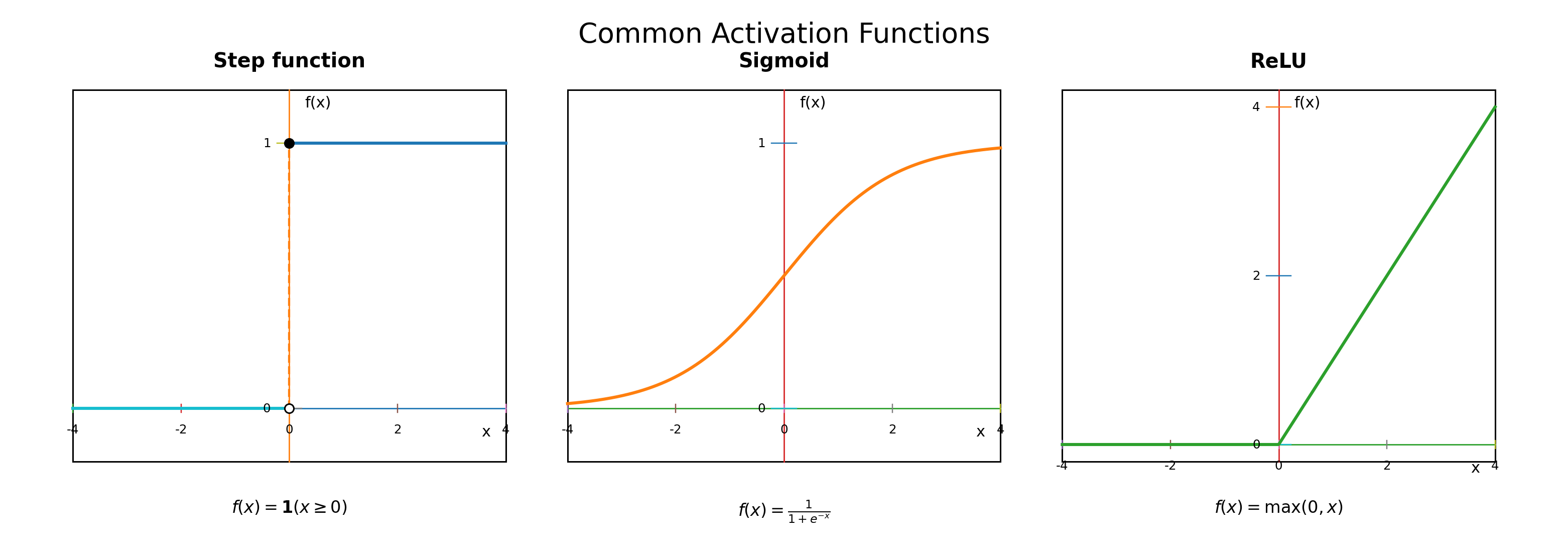
Weights are the most important part of a neural network. A weight is a number attached to each connection between units. If a weight is large and positive, the corresponding input strongly promotes activity. If the weight is negative, the input inhibits activity. If the weight is near zero, that input has little effect. If you have encountered regression in statistics, the concept is similar: in \(y = b_0 + b_1 x_1 + b_2 x_2\), the coefficients \(b_1\) and \(b_2\) tell you how much each predictor contributes. Weights play the same role. The key difference is that in regression the researcher interprets the coefficients; in a neural network, the weights are learned automatically from data. Bias is a constant added to the weighted sum before the activation function. It shifts the unit’s baseline response up or down, independent of the inputs, like an intercept in a regression. Activation functions determine what output the unit produces given its weighted sum. This is where non-linearity enters. Without a non-linear function, stacking multiple layers achieves nothing: a linear function of a linear function is still linear, so a deep network of linear units collapses mathematically to a single layer. Non-linearity breaks this limit. When you stack layers, each adding its own non-linearity, the network can represent increasingly complex relationships. Three common activation functions are:
- Step function: outputs 0 below threshold, 1 above. Used in the original perceptron, but the sharp jump makes it difficult to use with gradient-based learning.
- Sigmoid: a smooth S-curve between 0 and 1, interpretable as a probability. Standard in the 1980s and 1990s connectionist revival.
- ReLU (rectified linear unit): \(f(x) = \max(0, x)\). Here \(f(x)\) means “the output when the input is \(x\),” and \(\max(0, x)\) means “choose whichever is larger: 0 or \(x\).” So if \(x\) is positive, the function returns \(x\); if \(x\) is negative, it returns 0. Simple and effective; the most common activation function in modern networks.
Mathematically, the computation for one unit is:
\[s = \sum_{i=1}^{n} w_i x_i + b, \quad y = f(s)\]
where \(s\) is the weighted sum before activation, the symbol \(\sum\) means “add up,” \(i\) is just a counter that runs from 1 to \(n\), \(n\) is the number of inputs, \(w_i\) is the weight attached to input \(i\), \(x_i\) is input \(i\), \(b\) is the bias, \(y\) is the unit’s output, and \(f\) is the activation function.
In plain language: multiply each input by its weight, add those products together, add the bias, and then pass that total through the activation function to get the output.
Worked example: Suppose \(x_1 = 1\), \(x_2 = 0\), \(w_1 = 0.8\), \(w_2 = -0.4\), and \(b = 0.1\). The weighted sum is \(s = (0.8 \times 1) + (-0.4 \times 0) + 0.1 = 0.9\). With a sigmoid activation, the output is about 0.71. With a step activation at threshold 0, the output is 1. The same inputs produce different outputs depending on the activation function chosen.
Linking to psychological variables: These components connect to concrete research questions. Suppose the task is to classify whether a face is familiar. The inputs might be measurable features extracted from the face image, or behavioural measures such as response time and confidence. The output might be a binary decision (familiar or unfamiliar) or a continuous probability of familiarity. The weights determine how much each feature contributes to the decision, much as beta weights in multiple regression determine how much each predictor contributes. Learning, in this context, means adjusting weights so the network’s outputs move closer to the correct targets. (Rumelhart, McClelland, et al., 1986)
Layers: A full network stacks many units into layers. The input layer takes the raw data. The output layer produces the network’s answer. Between them are one or more , so called because their outputs are not directly observed. What do hidden layers compute? They compute features, measurable properties of the input that are useful for the task. A hidden unit combines several inputs (weighted and summed), applies a non-linear activation, and effectively creates a new feature that detects a particular pattern. For instance, one hidden unit might learn to respond to a diagonal edge; another to a colour gradient. These intermediate features are discovered during training, not specified by the designer.
The number of learnable parameters (weights and biases) grows quickly with the number of layers and units. A small network may have a few dozen parameters; a large language model can have hundreds of billions. This capacity allows the network to fit complex data, but it also raises the risk of : a network with enough parameters can memorise training data perfectly yet fail on new data. The practical challenge is building a model expressive enough to learn genuine structure but not so flexible that it memorises noise. (Goodfellow et al., 2016)
18.6 Learning and backpropagation
Learning requires two ingredients: a and an update rule.
18.6.1 Loss functions
The loss function (also called the error or cost function) measures how wrong the network’s current outputs are. It assigns a single number to performance: zero means perfect; larger values mean worse. It is the network’s only guide to learning. Two common choices:
- Mean squared error (MSE): for each training example, compute the squared difference between the network’s output and the correct answer, then average across all examples. If the network predicts 0.7 and the correct answer is 1.0, the squared error is \((0.7 - 1.0)^2 = 0.09\). MSE is standard for regression tasks.
- Cross-entropy: standard for classification. It penalises confident wrong answers heavily. If the network says it is 99% sure of the wrong category, cross-entropy assigns a very large loss; if it is only 51% sure, the loss is much smaller.
Entropy measures the average surprise in a set of outcomes: if a coin always lands heads, there is no surprise and entropy is zero; if it lands heads or tails with equal probability, surprise is high. Cross-entropy compares two probability distributions: the network’s predicted probabilities and the correct answers. It measures how surprised the network would be by the actual outcomes. High surprise means a large loss. Cross-entropy penalises confident wrong answers much more than hesitant ones, making it suited to classification tasks where the network outputs probabilities. (Goodfellow et al., 2016)
18.6.2 Gradient descent
Gradient descent uses derivatives to reduce the loss. For each weight, the algorithm asks: if I increase this weight by a tiny amount, does the loss go up or down? The derivative of the loss with respect to that weight gives the answer. If the derivative is positive, increasing the weight increases the loss, so the weight should decrease. If negative, the weight should increase. The learning rate controls how large each step is: too large and the network overshoots; too small and learning is slow.
A landscape analogy helps here: imagine the loss as the height of terrain and the current weights as a position on that terrain. Gradient descent rolls the ball downhill. At each step, it moves in the direction of steepest descent. Eventually it settles in a valley, a combination of weights where the loss is low. The procedure is not guaranteed to find the global lowest point; it may settle in a local minimum. In practice, though, gradient descent works well. (Rumelhart, Hinton, et al., 1986)
For mean squared error, the loss is:
\[L = \frac{1}{N} \sum_{i=1}^{N} (\hat{y}_i - y_i)^2\]
where \(L\) is the overall loss, \(N\) is the number of training examples, the hat in \(\hat{y}_i\) means “predicted value,” so \(\hat{y}_i\) is the model’s prediction for example \(i\), \(y_i\) is the correct answer for example \(i\), and \(\sum\) means add these squared errors across all examples before dividing by \(N\) to get the average.
In plain language: for each example, work out how far the prediction is from the correct answer, square that difference so that larger mistakes count more, and then average across all examples.
18.6.3 Backpropagation
Backpropagation (backward propagation of errors) makes gradient descent practical for multi-layer networks. The problem is that in a multi-layer network, we can measure error at the output layer, but how do we adjust weights in the hidden layers, which have no direct access to the correct answer? Backpropagation answers this using the chain rule from calculus. The chain rule is: if a change in \(A\) causes a change in \(B\), and a change in \(B\) causes a change in \(C\), then the effect of \(A\) on \(C\) can be computed by multiplying the two individual effects. The symbol \(\partial\) that appears below means a partial derivative: it tells us how much one quantity changes when we vary just one variable and hold the others fixed.
Applied to neural networks: the chain rule lets us trace the effect of each weight on the final loss, layer by layer. The algorithm works backward through the network. First, it computes the error at the output. Then it asks: how much did each weight in the last hidden layer contribute to that error? Then: how much did each weight in the second-to-last layer contribute? And so on, back to the first hidden layer. Each hidden unit receives a signal about how much it contributed to the overall error, and its weights are adjusted accordingly. The chain rule for a weight \(w\) can be written as:
\[\frac{\partial L}{\partial w} = \frac{\partial L}{\partial \hat{y}} \cdot \frac{\partial \hat{y}}{\partial s} \cdot \frac{\partial s}{\partial w}\]
where \(L\) is the loss, \(w\) is the weight we want to update, \(\hat{y}\) is the predicted output, \(s\) is the weighted sum before activation, and each fraction asks “how much does the top quantity change when the bottom quantity changes?” The dots mean multiply the three pieces together.
In plain language: this equation breaks a hard question, “how does this weight affect the loss?”, into three easier questions: how the loss depends on the prediction, how the prediction depends on the weighted sum, and how the weighted sum depends on the weight itself. Multiplying those pieces gives the weight’s contribution to the error. (Rumelhart, Hinton, et al., 1986)
Backpropagation is not a model of biological learning: it requires a global error signal and precise weight updates that are not obviously available to real neurons. It is, however, the standard algorithm in machine learning and the baseline for most deep learning systems.
18.6.4 Training, validation, and testing
Before training begins, available data are divided into three subsets:
- Training set: what the network learns from. Weights are adjusted to reduce loss on these examples.
- Validation set: never trained on directly. After each round of training, performance on the validation set is checked. This gives an independent measure of whether the network is learning the general pattern or memorising the training examples. The validation set is also used to choose hyperparameters, such as the number of layers, the learning rate, and the batch size. Hyperparameters are set by the researcher before training; they are distinct from the learned weights and biases.
- Test set: held back entirely until the end. Used once, to estimate performance on truly new data.
This separation matters because a network can achieve perfect performance on its training data and still fail on new data (overfitting). The validation set acts as an early warning: if training loss keeps decreasing but validation loss starts rising, the network is memorising rather than generalising, and training should stop. (Goodfellow et al., 2016)
18.6.5 Managing overfitting
Several techniques reduce overfitting:
- Early stopping: stop training when validation loss begins to rise.
- Weight decay: add a penalty for large weights, analogous to ridge regression (\(L2\) penalty) in statistics.
- Dropout: randomly turn off a fraction of units during training, forcing the network to build redundant representations and preventing reliance on any single unit.
- Data augmentation: create modified versions of training examples (flipping, rotating, or slightly distorting images) to expand the dataset. (Goodfellow et al., 2016)
18.6.6 Learning regimes
: the model is given input-output pairs and learns to predict the correct output. Covers classification and regression.
: inputs are given without labels and the model must discover structure. Relevant to perception because structure can emerge without explicit feedback.
: the model takes actions, receives rewards, and adjusts behaviour to maximise long-term reward. The learning signal is sparse and delayed, making credit assignment harder than in supervised learning. (Sutton & Barto, 2018)
For multi-class classification, a activation is used in the output layer. It converts raw output scores for all categories into probabilities that sum to 1:
\[p_j = \frac{e^{z_j}}{\sum_{i=1}^{k} e^{z_i}}\]
where \(p_j\) is the predicted probability of category \(j\), \(z_j\) is the raw score the network gives to category \(j\) before converting scores into probabilities, \(k\) is the total number of categories, \(\sum_{i=1}^{k}\) means add across all categories from 1 to \(k\), and \(e\) is a mathematical constant, approximately 2.718.
In plain language: softmax takes all the raw output scores, turns them into positive numbers, and rescales them so that the final probabilities across all categories add up to 1. The category with the highest probability is the network’s prediction.
18.7 Network types and what they are for
Neural networks come in several forms. The key distinctions are how information flows through the network and what kind of data it handles.
The simplest type is the single-layer perceptron, discussed above. It connects inputs directly to outputs with no hidden layers and can only learn linar classification boundaries.
A feedforward multi-layer network adds hidden layers and can represent non-linear functions. Information flows in one direction only: from input through hidden layers to output, with no loops or feedback. “Deep learning” refers to networks with many layers trained with backpropagation; “deep” means the number of hidden layers between input and output. (Rumelhart, Hinton, et al., 1986)
18.7.1 Convolutional neural networks
(CNNs) are designed for images and other data with spatial structure. A digital image is a grid of numbers; each pixel has a value for brightness or colour. The key idea is the convolutional filter (or kernel): a small grid of weights (for example, 3x3 or 5x5) that slides across the image, computing a weighted sum at each position. The same filter is applied at every location, so if the filter detects a vertical edge in the top-left corner, it can also detect vertical edges everywhere else. This weight sharing reduces the number of parameters compared to a fully connected network and makes the network tolerant of small position shifts: an edge is an edge, regardless of where it appears.
After convolution, pooling layers summarise local activity by taking the maximum or average value within small regions (e.g., 2x2 patches). This makes representations less sensitive to the exact position of features, a property called translation invariance that is important because objects can appear anywhere in an image.
CNNs learn feature hierarchies. Early layers detect simple features such as edges, corners, and colour gradients; middle layers combine those into textures, repeating patterns, and object parts; later layers respond to whole objects or categories. The network discovers this hierarchy on its own during training. This parallels Hubel and Wiesel’s work on the visual cortex in the 1960s, which showed that perception builds complex representations by composing simpler ones hierarchically. In the 2012 ImageNet challenge, AlexNet (designed by Krizhevsky, Sutskever, and Hinton) dramatically outperformed competing methods, reducing error by nearly half (Krizhevsky et al., 2012). Over the next few years, deep CNNs came to rival or surpass reported human baselines on some large-scale image-classification benchmarks, and that shift was a turning point for both research and industry.
For psychology, CNNs provide a testable model of visual processing. Researchers can ask: does the CNN confuse the same pairs of objects that humans confuse? Does it show the same difficulty with unusual viewpoints or poor lighting? Do activation patterns in its intermediate layers predict neural responses measured by fMRI? When answers are yes, it suggests the CNN has discovered computations similar to those used by the human visual system. When answers are no, it identifies where psychological theories of vision need further development. (Krizhevsky et al., 2012)
18.7.2 Recurrent neural networks
(RNNs) are designed for sequences: ordered data where position matters. Examples include words in a sentence, notes in a melody, eye fixations, or phonemes in a spoken word. The meaning of the current item depends on what came before: “bank” means something different after “river” than after “savings.”
Unlike feedforward networks, which process each input independently, RNNs have connections that loop back. At each time step, the network receives the current input and a copy of its previous hidden state, a running summary of everything seen so far. This hidden state acts as a memory. As each new input arrives, the hidden state is updated by combining the new input with the old state.
Standard RNNs have a practical weakness: they struggle with long-range dependencies. If relevant context is many steps in the past, information tends to fade or distort. Technically, gradients used in backpropagation either shrink to zero () or grow explosively (exploding gradients), making it hard to learn relationships across long sequences.
(LSTM) networks, invented by Hochreiter and Schmidhuber in 1997, solve this. The key innovation is a set of gates: learned mechanisms controlling information flow. An LSTM unit has three gates: an input gate (how much new information to let in), a forget gate (how much old memory to keep), and an output gate (how much stored memory to reveal). These gates allow the LSTM to selectively remember or forget, preserving important context across long sequences. LSTMs were the dominant architecture for sequence tasks for nearly two decades, until transformers began to replace them. (Hochreiter & Schmidhuber, 1997)
Psychological relevance: RNNs and LSTMs connect directly to working memory: the hidden state is a computational analogue of the active contents of working memory, carrying forward a representation of recent context that influences how new inputs are processed. The LSTM’s gating mechanism provides a model of how working memory might decide what to maintain and what to discard (interference management). Researchers have used these models to simulate serial recall, sentence processing, and sequential decision making. An LSTM trained to process sentences can learn to maintain subject-verb agreement across intervening clauses, a task that requires working memory in humans; when the model makes errors, they tend to be the same kinds of errors humans make. (Hochreiter & Schmidhuber, 1997)
18.7.3 Transformers
, introduced by Vaswani and colleagues in 2017, replace recurrence with . In an RNN, information must pass step by step from one time point to the next, and information can be lost along the way. Transformers take a different approach: every element in the sequence can “look at” every other element directly, in a single step. There is no chain of hidden states to pass information through.
The core mechanism is self-attention. For each token in a sequence, the model computes how much attention it should pay to every other token. In “The cat sat on the mat because it was tired,” when processing “it,” the model needs to determine that “it” refers to “the cat” rather than “the mat.” Self-attention allows the model to assign high attention weight to “cat” and low weight to “mat.” This is computed simultaneously for all tokens, which is much faster than stepping through the sequence one token at a time. The original transformer paper demonstrated that this architecture matched or exceeded RNN performance on machine translation while training faster. Transformers now underlie virtually all large language models. (Vaswani et al., 2017)
Psychological relevance: The word “attention” in the transformer literature differs from how psychologists typically use it, but there is a genuine parallel. In psychology, selective attention refers to focusing on relevant information while ignoring irrelevant information. In a transformer, attention is a learned mechanism that determines which parts of the context are relevant for processing the current input. Researchers can examine the attention patterns of a trained transformer and compare them to human eye-tracking data or reading-time measurements, asking whether the model and human focus on the same parts of a sentence. (Vaswani et al., 2017)
18.7.4 Reinforcement learning
Reinforcement learning (RL) is a different use of neural networks. In supervised learning, the network is told the correct answer for each example. In RL, there are no correct answers. Instead, an agent interacts with an environment, takes actions, and receives rewards. The agent must figure out through trial and error which actions lead to the best outcomes.
Consider training a network to play a computer game. The network sees the screen, chooses an action (e.g., move the paddle left, right, or stay), and receives a reward (e.g., points for breaking bricks, penalty for missing the ball). The network is not told which action is correct; it must discover through thousands of games that moving the paddle to meet the ball leads to better outcomes. This is learning from the consequences of actions.
The connection to psychology is direct: this is the behaviourist framework of Skinner’s operant conditioning, perhaps made more mathematically precise. (Sutton & Barto, 2018)
There are two key concepts here: the policy (a learned rule specifying what action to take in each state) and the value function (the estimated long-term payoff of being in a particular state, not just the immediate reward). Many RL algorithms learn both simultaneously. The value function helps the agent evaluate its situation (“How good is this state?”), while the policy determines what it does (“What action should I take?”). This maps onto a psychological distinction between evaluation (assessing how good an outcome is) and choice (selecting an action), which are thought to involve different neural systems.
Exploration versus exploitation: the agent must balance trying new actions against using actions that already seem good. This is a precise version of a problem that arises throughout human cognition. (Sutton & Barto, 2018)
18.8 Representation learning and distributed coding
A central idea in modern networks is . To understand it, consider two ways a neural system might represent information. In a localist representation, each concept is represented by a single unit or small group of dedicated units. Evidence exists in favour of this proposition: Quiroga and colleagues (2005) reported individual neurons in the human medial temporal lobe that responded selectively to specific people, one neuron firing when the patient saw pictures of Jennifer Aniston regardless of angle or context. This “Jennifer Aniston neuron” (or “grandmother cell”) suggests a localist code.
In a distributed representation, each concept is represented by a pattern of activity across many units, and each unit participates in representing many different concepts. “Dog” might be represented by a pattern where units 3, 7, 12, and 45 are highly active, while “cat” might be represented by a pattern where units 3, 7, 14, and 50 are active. The patterns overlap; both “dog” and “cat” share active units 3 and 7, which might encode features they share (four legs, fur, pet). This overlap is why distributed representations capture similarity: items similar in meaning have similar activation patterns.
This idea was central to the parallel distributed processing (PDP) tradition of Rumelhart, McClelland, and colleagues in the 1980s. Distributed representations have several advantages over localist ones: (1) the system captures similarity through pattern overlap; (2) it shows graceful degradation when units are damaged (because information is spread across many units, losing one unit degrades performance gradually rather than catastrophically); (3) it generalises to new items that share features with known items; and (4) it can represent many concepts using combinatorial patterns across a modest number of units, just as 26 letters can represent millions of words. (Rumelhart, McClelland, et al., 1986)
Lashley’s work in the 1920s through the 1950s anticipated this. He spent decades removing brain regions from rats, trying to localise memory. His conclusion was that memory is not localised in any single region but distributed across the cortex: removing any region degraded performance somewhat, but no single region was indispensable. In connectionist models, similarly, a memory is stored across many connection weights; damage to some units degrades the memory gradually but does not erase it, matching real brain behaviour better than localist models. (Rumelhart, McClelland, et al., 1986)
. A modern application of distributed representation is the embedding. An embedding represents an item (a word, a sentence, an image) as a vector of numbers in a multi-dimensional space. For example, the word “king” might be represented as a vector of 300 numbers learned during training by predicting words from their context in large bodies of text. The property of learned embeddings is that geometric relationships in the vector space correspond to semantic relationships. Words similar in meaning end up close together. Consistent relationships appear as consistent directions: the vector from “king” to “queen” is approximately the same as the vector from “man” to “woman.” Modern large language models represent every word (or sub-word token) as an embedding, and these embeddings are the foundation on which the model builds its understanding of language. Embeddings are not a complete theory of meaning, but they provide a concrete, computational framework for thinking about how meaning might be represented and compared. (Landauer & Dumais, 1997)
18.9 Psychological models that used networks
18.9.1 Face recognition: Bruce, Young, and Burton
In 1986, Vicki Bruce and Andrew Young proposed an information-flow model of face recognition. An information-flow model (sometimes called a “box-and-arrow” model) describes a cognitive process as a series of stages, each performing a different function. Bruce and Young proposed the following stages: structural encoding creates a representation of the face’s physical configuration; face recognition units (FRUs) compare this to stored representations of known faces; person identity nodes (PINs) link the recognised face to stored information about the person; and name generation retrieves the name. Separate parallel pathways handle emotional expression and facial speech (lip-reading). The model was supported by neuropsychological patients with selective impairments at different stages, and by the common experience of recognising a face without being able to recall the name. (Bruce & Young, 1986)
The Bruce and Young model was a verbal, box-and-arrow description. It specified the stages of face recognition but not the mechanisms: how does a face recognition unit actually match a perceived face to a stored representation? How fast does information flow between stages?
In 1990, Andrew Burton, Vicki Bruce, and Rob Johnston addressed these questions by implementing key parts of the Bruce and Young framework as an interactive activation and competition (IAC) network, where units are connected by excitatory and inhibitory links and activation spreads through the network over time. The move to a network model was motivated by precision: a working computational model generates quantitative predictions that a verbal description cannot.
In the IAC model, FRUs are connected to PINs by excitatory connections. When a face is perceived, its FRU becomes active and activation spreads to the corresponding PIN, which activates connected name and semantic information nodes. Connections are bidirectional: activation flows not only from FRU to PIN but also back. This reciprocal activation produces several predictions:
- Familiarity effects: familiar faces, which have strong FRU-to-PIN connections built through experience, produce faster and stronger activation than unfamiliar faces. This matches experimental findings.
- Semantic priming: having just seen Prince William leaves his PIN partially active, sending activation to associated PINs (e.g., King Charles). This makes it easier to recognise King Charles immediately after, an effect demonstrated in experiments.
- Competition: units at the same level inhibit each other, so the system settles on a single identification.
The specific architecture is less important than the general principle: a network model embodies a psychological theory, making its assumptions explicit and its predictions quantitative. A box-and-arrow model says “structural encoding feeds into face recognition units”; a network model specifies the connection strengths, the activation dynamics, and the time course, allowing researchers to simulate experiments and compare model behaviour to human data trial by trial. (Burton et al., 1990)
18.9.2 Past tense learning
Rumelhart and McClelland (1986) trained a connectionist network on English verb pairs and showed it could learn regular and irregular past tenses from examples alone, producing over-regularisation errors (such as “goed”) resembling children’s errors. The model suggested that rule-like behaviour could emerge from distributed representations without any symbolic rules. The network is trained on many verb pairs (walk/walked, go/went); it adjusts weights so that the output phonology matches the target past tense; it then produces over-regularisations when the statistical structure of the data favours regular patterns. (Rumelhart & McClelland, 1986)
Pinker and Prince (1988) challenged the model on several grounds: its phonological representations were unrealistic and contained encoding artefacts that inflated apparent success; the model could not handle certain linguistic distinctions (for example, the difference between “ring/rang” versus “wring/wringed”); and children’s over-regularisation errors do not follow the same statistical pattern as the model’s errors. Most fundamentally, Pinker and Prince argued that language requires rules: that regular past tenses are generated by a symbolic rule (“add -ed”) that is categorically different from memory-based retrieval of irregular forms. A single connectionist network, they argued, cannot capture this distinction. (Pinker & Prince, 1988)
The debate is instructive. The question is not merely “Does the model produce the right outputs?” but “Does it produce them for the right reasons, using mechanisms that match human behaviour in detail?” A model that gets answers right but makes the wrong kinds of errors is not a good psychological theory even if it is an effective engineering solution.
Symbolic versus connectionist: The past tense controversy reflects a broader debate. Symbolic theories propose that the mind operates on discrete symbols according to explicit rules; grammar, logical reasoning, and mathematical proof are naturally described this way. Connectionist theories propose that knowledge is stored implicitly in connection weights and that rule-like behaviour emerges from statistical regularities, without explicit rules. The dispute is not simply about which is correct; it is about what kind of explanation is adequate for different cognitive tasks. Many cognitive scientists now think the mind uses both types of processing, and the interesting question is which tasks use which kind of representation and how they interact. These models do not settle the debate, but a computational model forces a theory to specify mechanisms that can be tested against data. (Pinker & Prince, 1988; Rumelhart & McClelland, 1986)
18.10 Deep learning and scaling
The resurgence of neural networks depended on both algorithmic and hardware changes. Backpropagation provided a practical learning rule for multi-layer networks; later increases in computation made it possible to train larger models. Geoffrey Hinton, Yann LeCun, and Yoshua Bengio received the 2018 ACM Turing Award for their contributions to deep learning (Association for Computing Machinery, 2019a). Hinton and John Hopfield later shared the 2024 Nobel Prize in Physics for foundational discoveries and inventions that enable machine learning with artificial neural networks (Nobel Prize Outreach, 2024).
AlexNet’s 2012 ImageNet result was a turning point. Over the following years, training runs became much larger, datasets kept growing, and benchmark performance improved rapidly (OpenAI, 2018). This convinced both researchers and industry that deep learning was practically superior for many perceptual tasks, and investment in AI surged.
Source: ACM Turing Award lecture video. (Association for Computing Machinery, 2019b)
18.11 Transformers and large language models
18.11.1 Pretraining, fine-tuning, and tokens
To understand large language models (LLMs), several terms need to be defined.
A token is the basic unit the model processes. Tokens are not always whole words. Most LLMs use subword tokenisation, which breaks text into frequent chunks. For example, “unbelievable” might split into “un”, “believ”, and “able.” Common words like “the” are usually a single token. A rough rule of thumb is that one token is about three-quarters of a word in English.
Pretraining is the first and most expensive phase. The model is exposed to an enormous text corpus (billions or trillions of words scraped from books, websites, Wikipedia, code repositories, and other sources) and learns to predict text. Two main prediction objectives:
- Next-token prediction (GPT-style): given all the tokens so far, predict the next token. For example, given “The capital of France is”, predict “Paris.” This is done trillions of times, and the model gradually acquires grammar, facts, reasoning patterns, and style.
- Masked prediction (BERT-style): randomly hide some tokens in the input and predict the missing ones from the surrounding context. Because the model sees context on both sides of the masked token, this is a bidirectional objective.
is the second phase. The pre-trained model is further trained on a smaller, more specific dataset, for example a set of question-answer pairs to become a question-answering system, or on human feedback about helpfulness to become a better conversational assistant (a process called reinforcement learning from human feedback, RLHF). Fine-tuning is much cheaper and faster than pretraining because the model already knows a great deal about language. (Brown et al., 2020; Devlin et al., 2018)
18.11.2 Key models
BERT (Google, 2018): trained with bidirectional masked prediction; strong on comprehension tasks. Introduced the pre-training/fine-tuning pattern now standard across the field.
GPT-3 (OpenAI, 2020): 175 billion parameters, trained on next-token prediction. Its most notable feature was few-shot learning: given just a few examples in the prompt, it could perform a wide range of tasks without additional fine-tuning.
GPT-4 (OpenAI, 2023): multimodal (text and images), substantially better on benchmarks than earlier versions, including some professional and academic exams.
The landscape of LLMs has become crowded. Many other organisations have developed powerful models: Anthropic’s Claude, Meta’s LLaMA, Google’s Gemini, Mistral AI’s Mistral, and DeepSeek’s models. These differ in architecture details, training data, and design philosophy (for example, whether model weights are openly available), but all share the transformer architecture and the pre-training/fine-tuning approach. (Brown et al., 2020; OpenAI, 2023)
18.11.3 Prompting and in-context learning
GPT-3 demonstrated a notable capability: a model can adapt to new tasks from examples provided in the prompt, without any weight updates. This is called in-context learning. For example, including a few translation examples at the start of a prompt can cause the model to continue translating. It is not long-term learning (the model’s weights do not change), but it can adapt behaviour within a single conversation.
This gave rise to prompt engineering: the practice of crafting input prompts to elicit the best responses. Small changes in wording can produce different answers. Techniques include giving examples of desired outputs (“few-shot” prompting), asking the model to “think step by step” (chain-of-thought prompting), or assigning the model a role. (Brown et al., 2020)
18.11.4 Capabilities and limits
LLMs are effective at generating coherent text, summarising documents, translating, writing and debugging code, and answering questions. These abilities follow from the training objective: predicting the next token forces the model to represent grammar, facts, reasoning patterns, and style.
LLMs have a well-known failure mode: , producing fluent, confident text that is factually wrong. This is not a bug that can be easily patched; it is a consequence of how the models work. They generate the most probable continuation, which is not always the true one. A common example is fabricated academic references: a model asked to cite sources may generate realistic-looking author names, journal titles, and dates that correspond to no real publication.
“Temperature” controls how variable a model’s outputs are. At low temperature, the model tends to choose the most probable next token, producing safer, more predictable, and often more repetitive text. At high temperature, it more often selects less probable tokens, producing more varied and creative but also more error-prone text. The term does not refer to the machine’s physical temperature; it is simply the name given to this sampling parameter.
LLMs have a fixed context window: they can only use the tokens within it to generate responses. Long conversations or documents may exceed this limit. The models do not build long-term memories unless embedded in systems that store information externally. (Brown et al., 2020; OpenAI, 2023)
18.11.5 What LLMs offer psychology
LLMs provide a testbed for theories of language and cognition.
Surprisal and reading times: psycholinguists have established that less predictable words take longer to read. LLM token probabilities generate surprisal scores that predict human reading times well. This supports theories that human language processing is fundamentally predictive.
Semantic similarity: LLM embeddings predict how similar people judge two words or sentences to be. This supports distributed representation theories of meaning.
Syntactic processing: researchers test whether LLMs show the same sensitivity to grammatical structure as humans, for example subject-verb agreement across intervening clauses. When models succeed, it shows that statistical learning from text can capture syntactic structure; when they fail, it reveals what text alone cannot teach.
Cognitive biases: some studies have found that LLMs show human-like biases such as framing effects or anchoring. When they do, it suggests these biases may arise from statistical patterns in language rather than from specifically human cognitive architecture.
If a model trained only on text can approximate certain human behaviours, that tells us what can be learned from linguistic input alone. If it fails in systematic ways, that highlights what kinds of experience or structure might be missing: embodied experience, social interaction, visual grounding, or explicit reasoning. LLMs are best treated as baseline models: they show what statistical learning from text can achieve, which helps clarify what additional cognitive mechanisms humans might need. (Brown et al., 2020; OpenAI, 2023)
One approach is to treat LLMs as simulated experimental participants. Researchers present the model with the same stimuli used in human experiments (sentence completions, moral dilemmas, categorisation tasks) and compare model responses to human data. The point is not to claim the model is a person or has genuine understanding. Rather, the model serves as a null hypothesis: if statistical learning from text alone reproduces a human behavioural pattern, that pattern does not require more complex cognitive mechanisms. If the model fails, that tells us something important about what is missing from a purely statistical account.
18.12 Limits and evaluation
Neural networks are effective when the task is well specified and training data are sufficient. They do not constitute a general theory of cognition. They can approximate mathematical functions and produce impressive outputs, but they do not by themselves explain how humans understand meaning, set goals, or model other people’s beliefs and intentions. For psychology, neural networks are best treated as models to compare with human data, tools for generating precise predictions and identifying where theories succeed or fail, not as replacements for psychological theory. (OpenAI, 2023)
Models can be hard to interpret, and their outputs can be confident even when wrong. Evaluation means testing behaviour on new data and considering failure modes, not trusting the internal story the model seems to tell.
18.13 Criticisms of AI
The rapid development and deployment of AI systems has provoked serious criticism on multiple fronts.
Bias and discrimination. AI systems learn from data, and data reflect the world as it is, including its inequalities. If a facial recognition system is trained mainly on lighter-skinned faces, it will perform poorly on darker-skinned faces. If a hiring algorithm is trained on historical decisions, it may learn to discriminate against underrepresented groups because those groups were historically excluded. These are not hypothetical scenarios: studies have documented racial and gender biases in commercial facial recognition systems, language models, and hiring tools. The algorithm is not prejudiced; it faithfully reproduces statistical patterns in biased training data.
Environmental costs. Training large models consumes substantial energy and water. Training a single large language model can produce carbon emissions comparable to the lifetime emissions of several cars. As models grow larger and are trained more frequently, these costs increase.
Exploitative labour. Data labelling and content moderation, both necessary for AI systems, are often outsourced to workers in low-income countries who are paid low wages. Content moderation, reviewing harmful or disturbing material that AI systems produce or encounter, has been documented as causing psychological harm to the workers who perform it.
Intellectual property. LLMs and image generators are trained on material scraped from the internet, including copyrighted books, articles, artwork, and code. Artists, writers, and programmers have argued that using their work to train commercial AI systems without permission or compensation is ethically and legally wrong. Several lawsuits are testing whether this constitutes copyright infringement.
Deepfakes. AI can generate convincing fake images, audio, and video. These are already used for fraud, political disinformation, and non-consensual pornography.
Transparency and accountability. Deep neural networks are difficult to interpret. When a model makes a decision (denying a loan, flagging a person as high-risk, recommending a sentence), it may be impossible to explain why in terms a human can evaluate. Who is responsible when an AI system makes a harmful error?
Concentration of power. The development of the most capable AI systems requires enormous resources, concentrating influence in a small number of large companies, primarily in the United States and China. This raises concerns about monopolistic behaviour and the exclusion of smaller organisations and poorer countries from shaping a technology that will affect everyone.
These criticisms do not argue for abandoning AI. Many applications are genuinely beneficial. They do argue for critical engagement: technology is shaped by the decisions of the people who build, fund, and deploy it, and it carries the values and biases of its creators and their data.
18.14 Key terms
Activation function: A function applied to a unit’s weighted sum to determine its output. Non-linear activation functions give networks the ability to model complex relationships. Common types: sigmoid, ReLU, step function.
Attention mechanism: A component of neural networks (especially transformers) that allows each element in a sequence to selectively weight contributions from other elements by relevance. Enables modelling of long-range dependencies.
Backpropagation: The algorithm that computes how much each weight in a multi-layer network contributed to the overall error, using the chain rule from calculus. Allows gradient descent to update weights in all layers, not just the output layer.
Catastrophic forgetting: The tendency of a neural network to lose previously learned information when trained on new data. Contrasts with human memory, where new learning rarely erases old knowledge so completely.
Distributed representation: A scheme in which a concept is represented by a pattern of activity across many units rather than by a single dedicated unit. Allows similarity to be captured through pattern overlap and provides robustness to damage.
Embedding: A learned representation of an item (e.g., a word) as a vector of numbers in a multi-dimensional space. Items similar in meaning are represented by nearby vectors.
Gradient descent: An optimisation algorithm that adjusts each weight in the direction that reduces the loss function, using the derivative of the loss with respect to each weight.
Hebbian learning: A learning rule proposed by Donald Hebb (1949): when one neuron repeatedly contributes to the firing of another, the connection between them is strengthened. Often summarised as “neurons that fire together wire together.”
Large language model (LLM): A neural network (typically a transformer) with billions of parameters, pre-trained on vast text corpora to predict the next token. Examples: GPT-4, Claude, LLaMA, Gemini.
Perceptron: A single-layer neural network that multiplies inputs by weights, sums the results, and applies a threshold function to produce a binary output. Can learn linearly separable classification tasks. Invented by Frank Rosenblatt (1958).
Recurrent neural network (RNN): A neural network with connections that loop back, allowing it to maintain a hidden state across time steps. Designed for sequential data such as language, speech, and time series.
Reinforcement learning: A learning framework in which an agent interacts with an environment, takes actions, and receives rewards. The goal is to learn a policy that maximises long-term reward.
Transformer: A neural network architecture that uses self-attention instead of recurrence to process sequences. Underlies all modern large language models.
18.15 Short starting points
- Textbook-style intro (AI/NN overview): Goodfellow, Bengio, and Courville, Deep Learning, Chapter 1 (open online). (Goodfellow et al., 2016)
- Popular overview (non-technical): Mitchell, Artificial Intelligence: A Guide for Thinking Humans. (Mitchell, 2019)
- Brief online primer: CS50x AI notes overview. (CS50, 2026)